
This is actually an assignment from Jeremy Howard’s fast.ai course, lesson 5. I’ve showcased how easy it is to build a Convolutional Neural Networks from scratch using PyTorch. Today, let’s try to delve down even deeper and see if we could write our own nn.Linear module. Why waste your time writing your own PyTorch module while it’s already been written by the devs over at Facebook?
Well, for one, you’ll gain a deeper understanding of how all the pieces are put together. By comparing your code with the PyTorch code, you will gain knowledge of why and how these libraries are developed.
Also, once you’re done, you’ll have more confidence in implementing and using all these libraries, knowing how things work. There will be no myth to you.
And last but not least, you’ll be able to modify/tweak these modules should the situation require. And this is the difference between a noob and a pro.
OK, enough of the motivation, let’s get to it.
Simple MNIST one layer NN as the backdrop
First of all, we need some ‘backdrop’ codes to test whether and how well our module performs. Let’s build a very simple one-layer neural network to solve the good-old MNIST dataset. The code (running in Jupyter Notebook) snippet below:
# We'll use fast.ai to showcase how to build your own 'nn.Linear' module
%matplotlib inline
from fastai.basics import *
import sys

# create and download/prepare our MNIST dataset
path = Config().data_path()/'mnist'
path.mkdir(parents=True)
!wget http://deeplearning.net/data/mnist/mnist.pkl.gz -P {path}

# Get the images downloaded into data set
with gzip.open(path/'mnist.pkl.gz', 'rb') as f:
    ((x_train, y_train), (x_valid, y_valid), _) = pickle.load(f, encoding='latin-1')

# Have a look at the images and shape
plt.imshow(x_train[0].reshape((28,28)), cmap="gray")
x_train.shape

# convert numpy into PyTorch tensor
x_train,y_train,x_valid,y_valid = map(torch.tensor, (x_train,y_train,x_valid,y_valid))
n,c = x_train.shape
x_train.shape, y_train.min(), y_train.max()

# prepare dataset and create fast.ai DataBunch for training
bs=64
train_ds = TensorDataset(x_train, y_train)
valid_ds = TensorDataset(x_valid, y_valid)
data = DataBunch.create(train_ds, valid_ds, bs=bs)

# create a simple MNIST logistic model with only one Linear layer
class Mnist_Logistic(nn.Module):
    def __init__(self):
        super().__init__()
        self.lin = nn.Linear(784, 10, bias=True)

    def forward(self, xb): return self.lin(xb)

model =Mnist_Logistic()

lr=2e-2
loss_func = nn.CrossEntropyLoss()

# define update function with weight decay
def update(x,y,lr):
    wd = 1e-5
    y_hat = model(x)
    # weight decay
    w2 = 0.
    for p in model.parameters(): w2 += (p**2).sum()
    # add to regular loss
    loss = loss_func(y_hat, y) + w2*wd
    loss.requres_grad = True

    loss.backward()
    with torch.no_grad():
        for p in model.parameters():
            p.sub_(lr * p.grad)
            p.grad.zero_()
    return loss.item()

# iterate through one epoch and plot losses
losses = [update(x,y,lr) for x,y in data.train_dl]
plt.plot(losses);
These codes are quite self-explanatory. We used the fast.ai library for this project. Download the MNIST pickle file and unzip it, transfer it into a PyTorch tensor, then stuff it into a fast.ai DataBunch object for further training. Then we created a simple neural network with only one Linear layer. We also write our own update function instead of using the torch.optim optimizers since we could be writing our own optimizers from scratch as the next step of our PyTorch learning journey. Finally, we iterate through the dataset and plot the losses to see whether and how well it works.
First Iteration: Just make it work
All PyTorch modules/layers are extended from thetorch.nn.Module.
class myLinear(nn.Module):
Within the class, we’ll need an init dunder function to initialize our linear layer and a forward function to do the forward calculation. Let’s look at the init function first.
We’ll use the PyTorch official document as a guideline to build our module. From the document, an nn.Linear module has the following attributes:
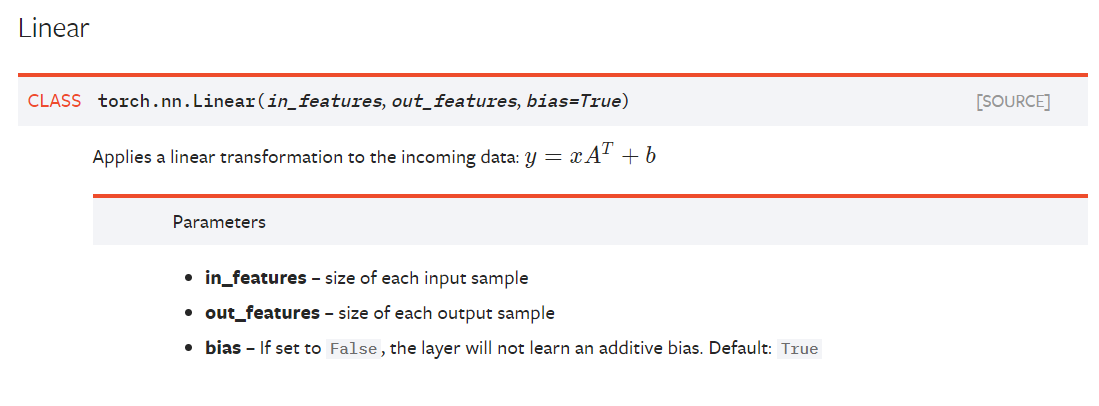
So we’ll get these three attributes in:
def __init__(self, in_features, out_features, bias=True):
        super().__init__()
        self.in_features = in_features
        self.out_features = out_features
        self.bias = bias
The class also needs to hold weight and bias parameters so it can be trained. We also initialize those.
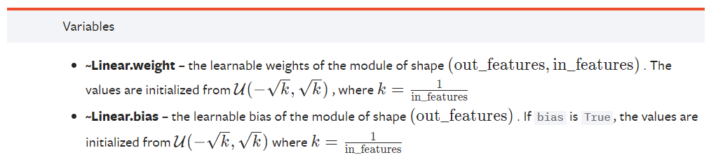
self.weight = torch.nn.Parameter(torch.randn(out_features, in_features))
self.bias = torch.nn.Parameter(torch.randn(out_features))
Here we used torch.nn.Parameter to set our weight and bias, otherwise, it won’t train.
Also, note that we used torch.randn instead of what’s described in the document to initialize the parameters. This is not the best way of doing weights initialization, but our purpose is to get it to work first, we’ll tweak it in our next iteration.
OK, now that the init part is done, let’s move on to forward function. This is actually the easy part:
def forward(self, input):
        _, y = input.shape
        if y != self.in_features:
            sys.exit(f'Wrong Input Features. Please use tensor with {self.in_features} Input Features')
        output = input @ self.weight.t() + self.bias
        return output
We first get the shape of the input, figure out how many columns are in the input, then check whether the input size match. Then we do the matrix multiplication (Note we did a transpose here to align the weights) and return the results. We can test whether it works by giving it some data:
my = myLinear(20,10)
a = torch.randn(5,20)
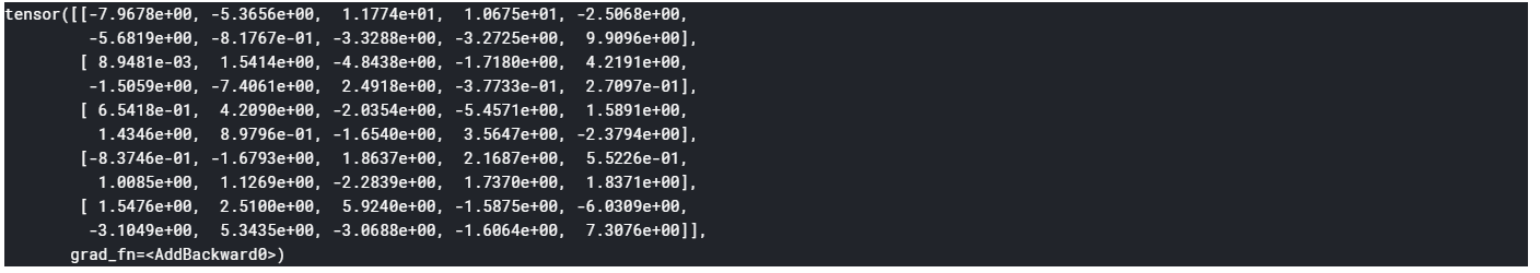
my(a)
We have a 5x20 input, it goes through our layer and gets a 5x10 output. You should get results like this:
OK, now go back to our neural network codes and find the Mnist_Logistic class, change self.lin = nn.Linear(784,10, bias=True) to self.lin = myLinear(784, 10, bias=True). Run the code, you should see something like this plot:
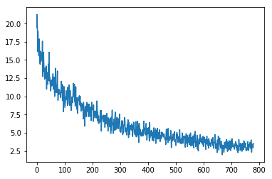
As you can see it doesn’t converge quite well (around 2.5 loss with one epoch). That’s probably because of our poor initialization. Also, we didn’t take care of the bias part. Let’s fix that in the next iteration. The final code for iteration 1 looks like this:
class myLinear(nn.Module):
    def __init__(self, in_features, out_features, bias=True):
        super().__init__()
        self.in_features = in_features
        self.out_features = out_features
        self.bias = bias
        self.weight = torch.nn.Parameter(torch.randn(out_features, in_features))
        self.bias = torch.nn.Parameter(torch.randn(out_features))


    def forward(self, input):
        x, y = input.shape
        if y != self.in_features:
            sys.exit(f'Wrong Input Features. Please use tensor with {self.in_features} Input Features')
        output = input @ self.weight.t() + self.bias
        return output
Second iteration: Proper weight initialization and bias handling
We’ve handled init and forward, but remember we also have a bias attribute that if False, will not learn additive bias. We have not implemented that yet. Also, we used torch.nn.randn to initialize the weight and bias, which is not optimum. Let’s fix this. The updated init function looks like this:
def __init__(self, in_features, out_features, bias=True):
        super().__init__()
        self.in_features = in_features
        self.out_features = out_features
        self.bias = bias
        self.weight = torch.nn.Parameter(torch.Tensor(out_features, in_features))
        if bias:
            self.bias = torch.nn.Parameter(torch.Tensor(out_features))
        else:
            self.register_parameter('bias', None)

        self.reset_parameters()
First of all, when we create the weight and bias parameters, we didn’t initialize them as the last iteration. We just allocate a regular Tensor object to it. The actual initialization is done in another function reset_parameters(will explain later).
For bias, we added a condition that if True, do what we did the last iteration, but if False, will use register_parameter(‘bias’, None) to give it None value. Now for reset_parameter function, it looks like this:
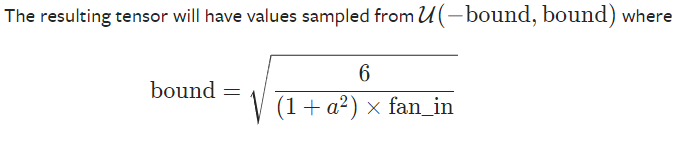
def reset_parameters(self):
        torch.nn.init.kaiming_uniform_(self.weight, a=math.sqrt(5))
        if self.bias is not None:
            fan_in, _ torch.nn.init._calculate_fan_in_and_fan_out(self.weight)
            bound = 1 / math.sqrt(fan_in)
            torch.nn.init.uniform_(self.bias, -bound, bound)
The above code is taken directly from PyTorch source code. What PyTorch did with weight initialization is called kaiming_uniform_. It’s from a paper Delving deep into rectifiers: Surpassing human-level performance on ImageNet classification — He, K. et al. (2015).
What it actually does is by initializing weight with a normal distribution with mean 0 and variance bound, it avoids the issue of vanishing/exploding gradients issue(though we only have one layer here, when writing the Linear class, we should still keep MLN in mind).
Notice that for self.weight, we actually give the a a value of math.sqrt(5) instead of the math.sqrt(fan_in) , this is explained in this GitHub issue of PyTorch repo for whom might be interested.
Also, we can add some extra_repr string to the model:
def extra_repr(self):
        return 'in_features={}, out_features={}, bias={}'.format(
            self.in_features, self.out_features, self.bias is not None
        )
The final model looks like this:
class myLinear(nn.Module):
    def __init__(self, in_features, out_features, bias=True):
        super().__init__()
        self.in_features = in_features
        self.out_features = out_features
        self.bias = bias
        self.weight = torch.nn.Parameter(torch.Tensor(out_features, in_features))
        if bias:
            self.bias = torch.nn.Parameter(torch.Tensor(out_features))
        else:
            self.register_parameter('bias', None)
        self.reset_parameters()

    def reset_parameters(self):
        torch.nn.init.kaiming_uniform_(self.weight, a=math.sqrt(5))
        if self.bias is not None:
            fan_in, _ = torch.nn.init._calculate_fan_in_and_fan_out(self.weight)
            bound = 1 / math.sqrt(fan_in)
            torch.nn.init.uniform_(self.bias, -bound, bound)

    def forward(self, input):
        x, y = input.shape
        if y != self.in_features:
            print(f'Wrong Input Features. Please use tensor with {self.in_features} Input Features')
            return 0
        output = input.matmul(weight.t())
        if bias is not None:
            output += bias
        ret = output
        return ret

    def extra_repr(self):
        return 'in_features={}, out_features={}, bias={}'.format(
            self.in_features, self.out_features, self.bias is not None
        )
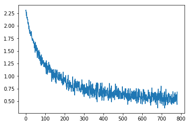
Rerun the code, you should be able to see this plot:
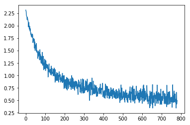
We can see it converges much faster to a 0.5 loss in one epoch.
Conclusion
I hope this helps you clear the cloud on these PyTorchnn.modules a bit. It might seem boring and redundant, but sometimes the fastest( and shortest) way is the ‘boring’ way. Once you get to the very bottom of this, the feeling of knowing that there’s nothing ‘more’ is priceless. You’ll come to the realization that:
Underneath PyTorch, there’s no trick, no myth, no catch, just rock-solid Python code.
Also by writing your own code, then compare it with official source code, you’ll be able to see where the difference is and learn from the best in the industry. How cool is that?